The World Income Inequality Database (WIID) contains information about income inequality for 201 countries. WIID updates without a specific schedule. The current version, released on 28 November 2023, contains over 24,000 data points with observations from pre-1960s to 2022. We will import this dataset from the downloaded .xlse file from its website (https://www.wider.unu.edu/database/world-income-inequality-database-wiid).
WIID combines information from various authoritative sources including:
LIS Cross-National Data Center (Luxembourg Income Study)
Eurostat
Socio-Economic Database for Latin America and the Caribbean (SEDLAC)
United Nations
Household survey statistics obtained from national statistical offices of the corresponding countries
Organisation for Economic Co-operation and Development (OECD)
World Bank’s Poverty and Inequality Platform (PIP)
Research outputs such as journal articles
Other international organizations
The observations are distributed across time periods as follows:
Time span
Number of observations
Total observations
24,367
Before 1960
311
1960-69
714
1970-79
946
1980-89
1,651
1990-99
3,758
2000-09
6,764
2010-19
8,753
2020-
1,470
2.2 2.2 Missing value analysis
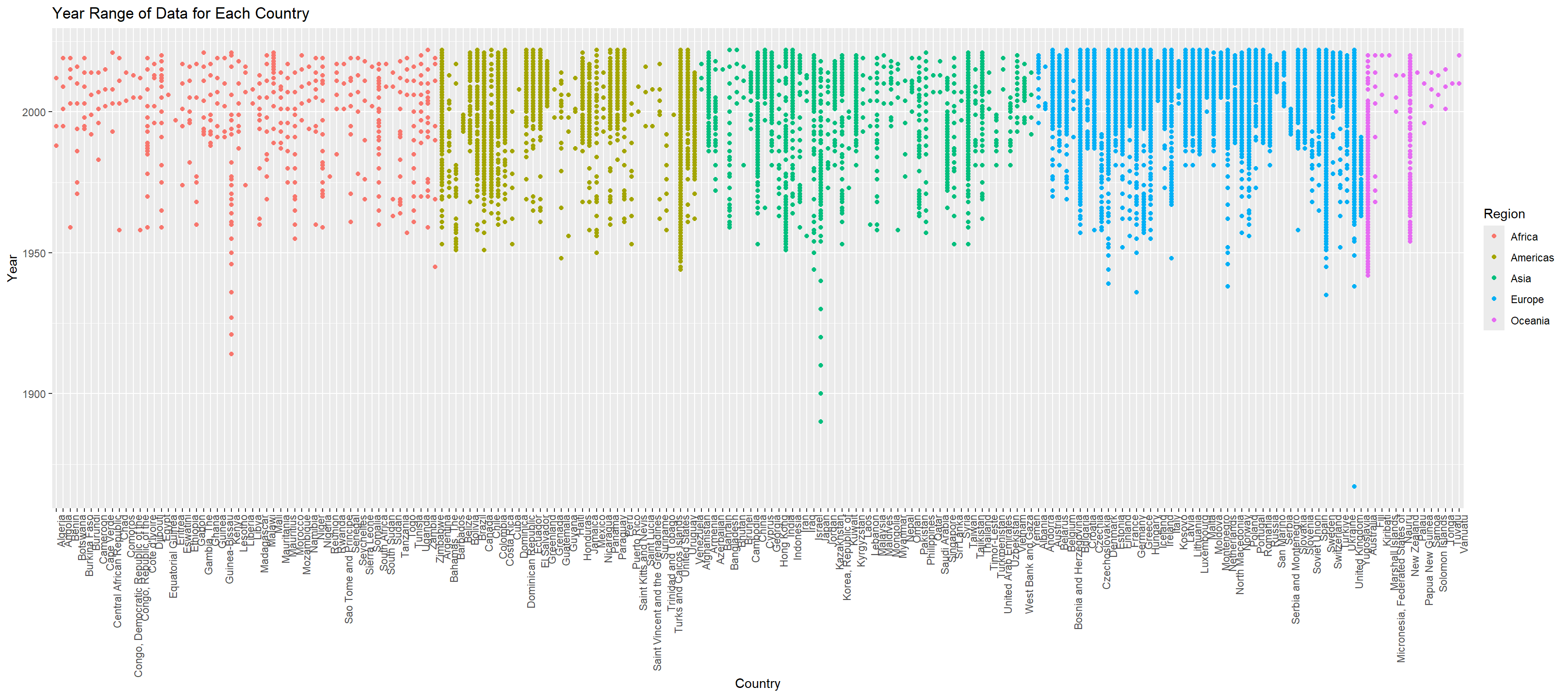
We want to first look at the range of years for the data by country and by continent to see if we can observe any patterns.
We observe that region NA only contains one contry Turkiye, so we decide to categorize it into Europe
Code
library(readxl)
Warning: package 'readxl' was built under R version 4.4.2
Code
library(ggplot2)library(tidyverse)
── Attaching core tidyverse packages ──────────────────────── tidyverse 2.0.0 ──
✔ dplyr     1.1.4     ✔ readr     2.1.5
✔ forcats   1.0.0     ✔ stringr   1.5.1
✔ lubridate 1.9.3     ✔ tibble    3.2.1
✔ purrr     1.0.2     ✔ tidyr     1.3.1
── Conflicts ────────────────────────────────────────── tidyverse_conflicts() ──
✖ dplyr::filter() masks stats::filter()
✖ dplyr::lag()    masks stats::lag()
ℹ Use the conflicted package (<http://conflicted.r-lib.org/>) to force all conflicts to become errors
Code
data <-read_excel("WIID_28NOV2023.xlsx")data <- data |>mutate(region_un =ifelse(country =="Turkiye", "Europe", region_un))
Code
data <- data |>mutate(country =factor(country, levels = data |>distinct(country, region_un) |>arrange(region_un, country) |>pull(country)))# Create the plot without connecting points and retaining multiple data points per countryggplot(data, aes(x = country, y = year, color = region_un)) +geom_point() +theme(axis.text.x =element_text(angle =90, hjust =1)) +labs(title ="Year Range of Data for Each Country", x ="Country", y ="Year", color ="Region")
From the plot, we can observe that even though the data spans over 100 years, most records are concentrated between the 1950s and 2020s. We can also see that countries in Europe and America have the most frequent data recordings, with almost a data point for each year. Whereas for African countries, data are measured less frequently.
Code
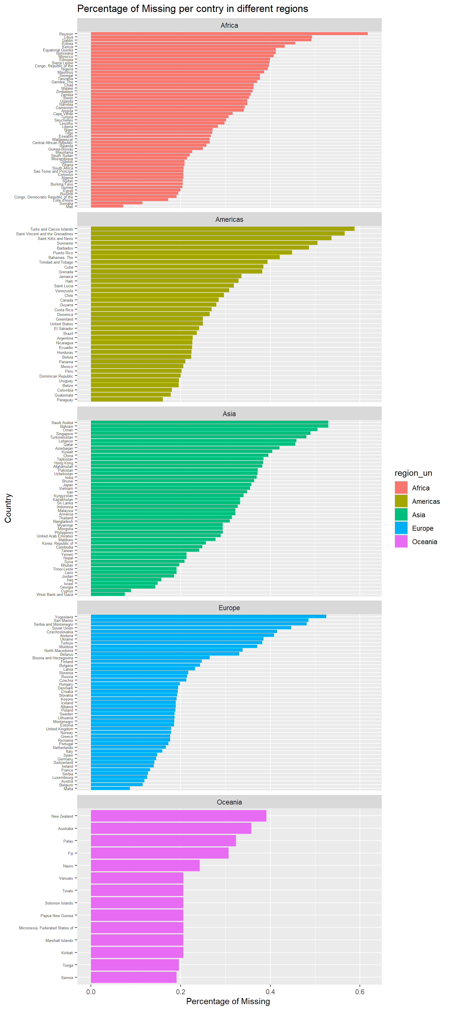
Data <-read_xlsx("WIID_28NOV2023.xlsx")colnum <-ncol(Data)Data |>mutate(total_missing =rowSums(is.na(Data))) |>group_by(country)|>mutate(rownum =n()) |>ungroup() |>group_by(region_un,country) |>summarize(missing=sum(total_missing)/(unique(rownum)*colnum)) |>ungroup() |>mutate(region_un=if_else(country=="Turkiye","Europe",region_un))|>ggplot(aes(y=fct_reorder(country,missing),x=missing,fill=region_un))+geom_col()+theme(axis.text.y =element_text(size =5)) +labs(x="Percentage of Missing ",y="Country",title ="Percentage of Missing per contry in different regions") +facet_wrap(~region_un,ncol=1,scales ="free_y")
`summarise()` has grouped output by 'region_un'. You can override using the
`.groups` argument.
From the plot facet by region_un, The missing data percentages vary significantly across different regions, with some regions having higher proportions of missing values. In Africa,a wide range of missing percentages with some countries having very high percentages (close to 50% or more), which suggests potential challenges in data collection or reporting consistency in this region.
In Asia, countries generally have moderate to low missing data percentages, while a few countries have higher percentages.
In Americas and Europe, lower percentage of countries contains high percentage of missing values while smaller countries and island nations have slightly higher missing percentages, which is consistent with the insight from the last graph where Americas and Europe has fewer challenges in data collection and report the data more frequently. In Oceania, smaller amount of countries belong to this region and most of them have relatively lower missing percentages, which means data availability are better in this developed countries.